Using GNURadio Companion To Visualize A Filter Response

 

You can quickly visualize a filter response in GNURadio by just hooking up a Gaussian Noise Source block to the filter input and applying a QT Frequency Sink to the output. Turning on the frequency sinks’s Averaging to ‘High’ helps to smooth out the resulting curve. Setting the QT Frequency Sink's 'Window' type to 'Blackman', and FFT Size to a large number helps in visualizing the filters fine detail.

 

Figure 1 - To test the frequency response of a filter, just feed it with noise and look at the result with a QT Frequency Sink block. As shown above the filter to be tested (circled in red) is fed from a noise source and the output is fed to a QT Frequency Sink.

 

Figure 2 - The resulting ‘frequency response’ is still noisy, but you can clearly see the results and judge how well your design meets the design specifications.

 

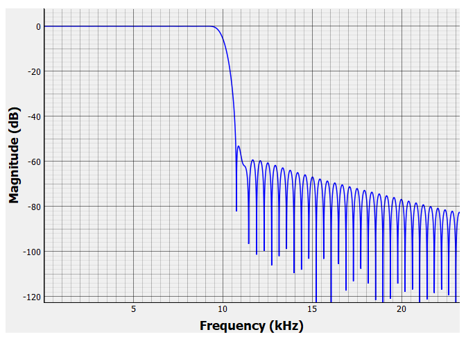
Figure 3 - Comparing the 'Tested' response of figure 2 with the GNURadio Filter Design Tool's calculated response for the same filter (above) shows good correlation. But it is not always easy to translate the GNURadio Companion Filter Blocks designs to the underlying Filter Design Tools parameters. It is much quicker to test any filter as per figure 1.

Bonus

If you are going to make a graph like figure 2, and want the passband to be normalized to 0 dB. Just read the value you are getting (approximately -52 dB in figure 2), then converting this to volts gives 398 (398 = 10^(52/20)). Change the noise sources 'Amplitude' to 398 and your plot will be normalized to 0 dB in the passband. This setting is valid for any subsequent sample rate, but changing the FFT size in the QT Frequency Sink will require a new normalizing factor.